18 Grammar of layered graphics I
You’ve made it quite far through this book. Now, I want to bring us back to the very beginning. In the first chapter we created a few visualizations with ggplot2. I want to unpack ggplot2 a bit more and also address some of the more philosophical underpinnings of visualization.
This chapter introduces you to the idea of the grammar of graphics, discusses when which visualizations are appropriate, and some fundamental design principles follow.
18.1 The Grammar of Layered Graphics
The gg in ggplot2 refers to the grammar of graphics (and the 2 is because it’s the second iteration). The Grammar of Graphics (Wilkinson, 1999) is a seminal book in data visualization for the sciences in which, Wilkinson defines a complete system (grammar) for creating visualizations that go beyond the standard domain of “named graphics”—e.g. histogram, barchart, etc.5960
ggplot2 is “an open source implementation of the grammar of graphics for R.”61 Once we can internalize the grammar of graphics, creating plots will be an intuitive and artistic process rather than a mechanical one.
There are five high level components of the layered grammar62. We will only cover the first two in this chapter.
-
Defaults:
- Data
- Mapping
-
Layers:
- Data*
- Mapping*
- Geom
- Stat
- Position
- Scales
- Coordinates
- Facets
18.2 Layers and defaults
Let’s first set up our package environment. We will use the commute dataset again.
In the first chapter of this section we explored these principles but did not put a name to them. Recall that we can use ggplot() by itself and it returns a chart of nothing.
ggplot()
This is because we have not specified any of the defaults. In order for us to plot anything at all, we need to specify what (the data object) will be visualized, which features (the aesthetic mappings), and how (the geoms). When we begin to specify our x and y aesthetics the scales are interpreted.
ggplot(commute, aes(med_house_income, by_auto))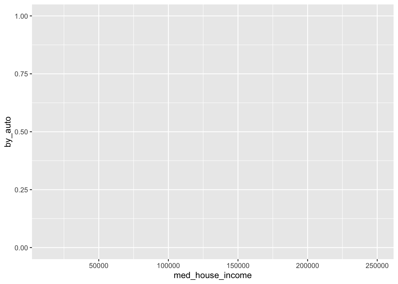
The final step is to add the geom layer which will inherit the data, aesthetic mappings, scale, and position while the geom_*() layer dictates the geometry.
ggplot(commute, aes(bach, med_house_income))+
geom_point()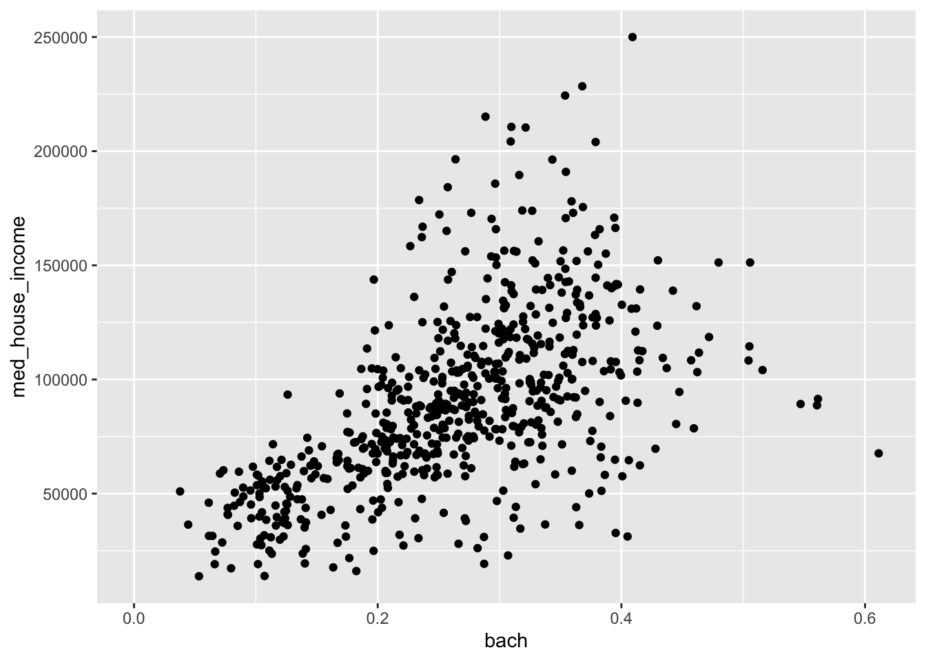
While this is the most common way you might define a ggplot, you should also be aware of the fact that each layer can stand on its own without you defining any of the defaults in the ggplot() call. Each geom inherits the defaults from ggplot(), but each geom_*() also has arguments for data, and mapping, providing you with increased flexibility.
Note: the
geom_*()s have the data as the second argument so either put the data there or name the argument explicitly. The choice is yours. Choose wisely!
What happens if we provide all of this information to geom_point() and entirely omit ggplot()?
geom_point(aes(med_house_income, by_auto), commute)
#> mapping: x = ~med_house_income, y = ~by_auto
#> geom_point: na.rm = FALSE
#> stat_identity: na.rm = FALSE
#> position_identityWe see that we do not have the plot, but we do have all of the information required of a layer is printed out to the console. If we add an empty ggplot call ahead of the layer, we will be able to create the plot.
ggplot() +
geom_point(aes(med_house_income, by_auto), commute)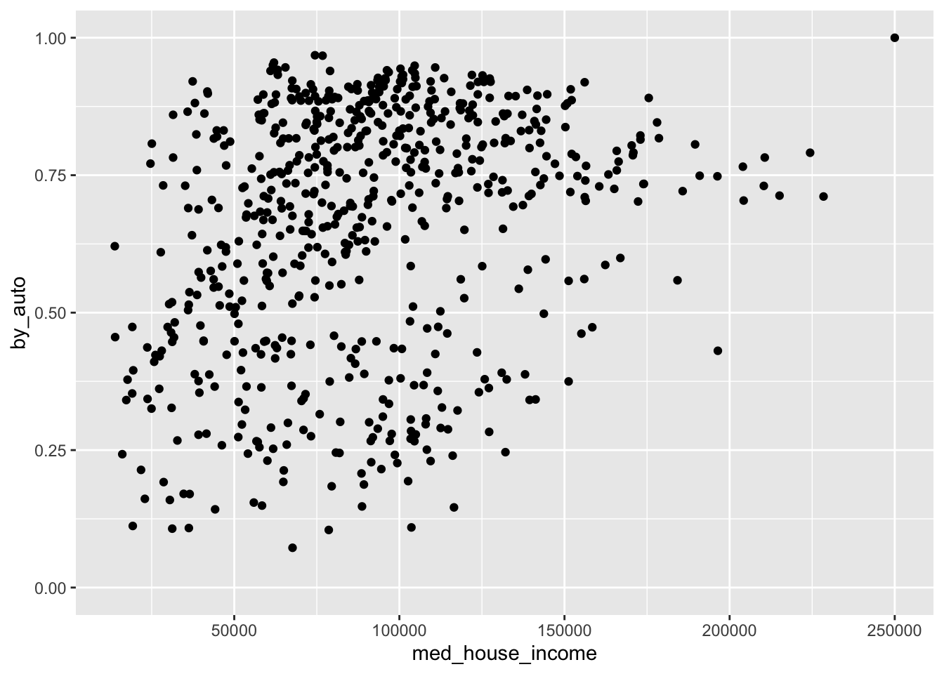
Being able to specify different data objects within each layer will provie to be extraordinarily helpful when we begin to work with spatial data, or plotting two different data frames with the same axes, or any other creative problem you wish to solve.